10. Navigating a Pivot Table
Chris Bailiss
2023-10-01
Source:vignettes/v10-navigatingapivottable.Rmd
v10-navigatingapivottable.RmdIn This Vignette
- High Level Methods vs. Low Level Methods
- Navigating Data Groups
- Navigating Cells
- Navigating between data groups and rows / columns / cells
High Level Methods vs. Low Level Methods
Most of the previous vignettes have utilised “high-level” methods to relatively quickly build a pivot table with a minimum of code and without having to worry about low-level structures and layout. Such high-level methods include:
-
qpvt(),qhpvt()andqlpvt()to build and output an entire pivot table in a single function call. -
pt$addColumnDataGroups()andpt$addRowDataGroups()- to add multiple column/row data groups in a single method call. -
pt$evaluatePivot()- to execute all of the following if they have not yet been executed:-
pt$normaliseColumnGroups()- to ensure all of the column data groups have the same depth. -
pt$normaliseRowGroups()- to ensure all of the row data groups have the same depth. -
pt$generateCellStructure()- to generate the (uncalculated) cells. -
pt$evaluateCells()- to calculate the cells.
-
-
pt$renderPivot()- to executept$evaluatePivot()if not already executed and then output the pivot table as an htmlwidget. -
pt$findColumnDataGroups()andpt$findRowDataGroups()to select data groups matching specific criteria in a single method call. -
pt$getCells()andpt$findCells()to select cells matching specific criteria in a single method call.
All of the above methods serve to make creating or navigating a pivot table quicker and easier in most circumstances.
Sometimes however, a more unusual or complex pivot table needs
creating or more granular navigation of the pivot table structures is
needed. The pivottabler package includes a set of
lower-level methods to create and navigate a pivot table. Using these
methods provides more flexibility but also requires more effort and more
lines of code than using the high-level methods above.
This vignette describes the set of low-level methods for navigating a pivot table.
The Irregular Layout vignette describes the low-level methods for creating a pivot table.
Navigating Data Groups
Example Pivot Table
The following pivot table will be used as the basis of the examples in this section:
library(pivottabler)
createPivot1 <- function() {
  pt <- PivotTable$new()
  pt$addData(bhmtrains)
  pt$addColumnDataGroups("TrainCategory")
  pt$addColumnDataGroups("PowerType")
  pt$addRowDataGroups("TOC")
  pt$defineCalculation(calculationName="TotalTrains", summariseExpression="n()")
  return(pt)
}
pt <- createPivot1()
pt$renderPivot()
Data Group Class
Each data group is an instance of the PivotDataGroup
class. See the Class Overview appendix
for details.
Data Group Hierarchy
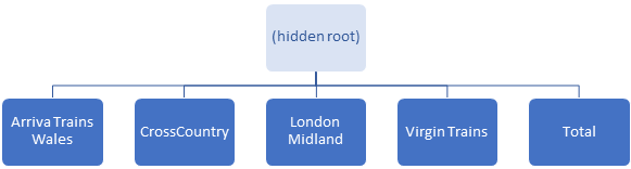
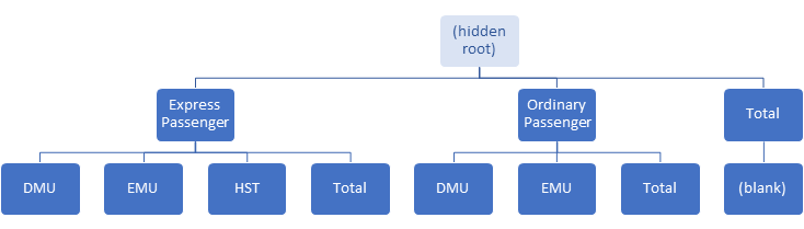
Two sets of data groups exist in a pivot table - one on each axis, i.e. on rows and on columns. Each set of data groups exists in a hierarchy. Each hierarchy starts with a single hidden root data group on each axis.
For example, considering the hierarchy of data groups on the rows axis and columns axis:
The hidden root data groups are normally rarely explicitly used,
though we will use them in some examples in this vignette. They can be
accessed using pt$columnGroup and
pt$rowGroup.
Data Group Parents and Children
Every data group can have a set of child data groups. Use
childGroupCount to count the child groups:
pt$rowGroup$childGroupCount## [1] 5
pt$columnGroup$childGroupCount## [1] 3The child groups are accessed via the childGroups
property, which returns an R list containing the data groups directly
below this group in the hierarchy.
Every data group, except the hidden root data group on each axis,
will have a parent data group, accessed via the parentGroup
property.
Retrieving the caption of the first visible row group:
pt$rowGroup$childGroups[[1]]$caption## [1] "Arriva Trains Wales"Retrieving the caption and child count of the second visible column group:
pt$columnGroup$childGroups[[2]]$caption## [1] "Ordinary Passenger"
pt$columnGroup$childGroups[[2]]$childGroupCount## [1] 3Retrieving the first child of this group:
pt$columnGroup$childGroups[[2]]$childGroups[[1]]$caption## [1] "DMU"Highlighting these three data groups:
pt <- createPivot1()
pt$setStyling(groups=pt$rowGroup$childGroups[[1]], declarations=list("background-color"="yellow"))
pt$setStyling(groups=pt$columnGroup$childGroups[[2]], declarations=list("background-color"="cyan"))
pt$setStyling(groups=pt$columnGroup$childGroups[[2]]$childGroups[[1]],
              declarations=list("background-color"="lawngreen"))
pt$renderPivot()
We can even navigate down and back up the hierarchy:
pt$columnGroup$childGroups[[2]]$childGroups[[1]]$parentGroup$caption## [1] "Ordinary Passenger"Data Group Levels
The first level of visible data groups is referred to as level 1, the second level as level 2, etc. Another way of referring to the levels is “top-level”, which refers to level 1 and “leaf-level” which refers to the bottom level, which has the highest level number.
The level number of an individual data group can be retrieved using
the levelNumber property.
pt$rowGroup$childGroups[[1]]$levelNumber## [1] 1
pt$columnGroup$childGroups[[2]]$childGroups[[1]]$levelNumber## [1] 2To count the number of levels of groups use
pt$rowGroupLevelCount or
pt$columnGroupLevelCount:
pt$rowGroupLevelCount## [1] 1
pt$columnGroupLevelCount## [1] 2To get the row groups at a particular level use
pt$getRowGroupsByLevel():
grps <- pt$getRowGroupsByLevel(1)
fx <- function(x) { x$caption }
sapply(grps, fx)
## [1] "Arriva Trains Wales" "CrossCountry" "London Midland"
## [4] "Virgin Trains" "Total"Similarly, to get the column groups at a particular level use
pt$getColumnGroupsByLevel():
grps <- pt$getColumnGroupsByLevel(2)
fx <- function(x) { x$caption }
sapply(grps, fx)
## [1] "DMU" "EMU" "HST" "Total" "DMU" "EMU" "Total" ""Top Level Groups
In the examples above, pt$rowGroup$childGroups was used
to retrieve the top-level row groups, and
pt$columnGroup$childGroups was used to retrieve the
top-level column groups. An easier way to retrieve these groups is
pt$topRowGroups and pt$topColumnGroups:
fx <- function(x) { x$caption }
grps <- pt$topRowGroups
sapply(grps, fx)
## [1] "Arriva Trains Wales" "CrossCountry" "London Midland"
## [4] "Virgin Trains" "Total"
grps <- pt$topColumnGroups
sapply(grps, fx)
## [1] "Express Passenger" "Ordinary Passenger" "Total"Ancestors, Descendants and Leaves
Example Pivot Table
The following pivot table will be used in the next few examples:
library(dplyr)
library(pivottabler)
createPivot2 <- function() {
  trains <- filter(bhmtrains, (TOC=="CrossCountry")|(TOC=="Virgin Trains"))
  pt <- PivotTable$new()
  pt$addData(trains)
  pt$addRowDataGroups("TOC")
  pt$addRowDataGroups("TrainCategory", addTotal=FALSE)
  pt$addRowDataGroups("PowerType", addTotal=FALSE)
  pt$defineCalculation(calculationName="Train Count", summariseExpression="n()")
  return(pt)
}
pt <- createPivot2()
pt$renderPivot()
Ancestors
Consider the “HST” data group:
pt <- createPivot2()
grp <- pt$topRowGroups[[1]]$childGroups[[1]]$childGroups[[2]]
pt$setStyling(groups=grp, declarations=list("background-color"="yellow"))
pt$renderPivot()
The ancestors of this group are the groups above it in the hierarchy,
i.e. parent group, grandparent group, etc. The ancestors can be
retrieved using getAncestorGroups() which returns a list of
data groups:
pt <- createPivot2()
grp <- pt$topRowGroups[[1]]$childGroups[[1]]$childGroups[[2]]
pt$setStyling(groups=grp, declarations=list("background-color"="yellow"))
ancestors <- grp$getAncestorGroups()
pt$setStyling(groups=ancestors[[1]], declarations=list("background-color"="cyan"))
pt$setStyling(groups=ancestors[[2]], declarations=list("background-color"="lawngreen"))
pt$renderPivot()
Descendants
Consider the “CrossCountry” data group:
pt <- createPivot2()
grp <- pt$topRowGroups[[1]]
pt$setStyling(groups=grp, declarations=list("background-color"="yellow"))
pt$renderPivot()
The descendants of this group are all of the groups below it in the
hierarchy, i.e. children, grandchildren, etc. The descendants can be
retrieved using getDescendantGroups() which also returns a
list of data groups:
Leaves
The “leaves” of the “CrossCountry” group are all of the groups below
it at the lowest level in the hierarchy. The “leaves” can be retrieved
using getLeafGroups() which also returns a list of data
groups:
pt <- createPivot2()
grp <- pt$topRowGroups[[1]]
pt$setStyling(groups=grp, declarations=list("background-color"="yellow"))
descendants <- grp$getLeafGroups()
pt$setStyling(groups=descendants, declarations=list("background-color"="cyan"))
pt$renderPivot()
It is also possible to retrieve all of the the leaf groups on either
the rows or columns axes using pt$leafRowGroups or
pt$leafColumnGroups:
All groups on an axis
All of the groups on either axis can be retrieved using
pt$allRowGroups or pt$allColumnGroups:
pt <- createPivot1()
grps <- pt$allRowGroups
pt$setStyling(groups=grps, declarations=list("background-color"="yellow"))
grps <- pt$allColumnGroups
pt$setStyling(groups=grps, declarations=list("background-color"="cyan"))
pt$renderPivot()
In the above pivot table there is only one level of row data groups
so pt$topRowGroups, pt$leafRowGroups and
pt$allRowGroups all return the same set of groups.
Outline group relationships
Outline groups (see the Regular Layout vignette) are usually created in sets of two or three groups. For example, consider the following pivot table, where three rows are created for each train operating company (TOC):
library(dplyr)
library(pivottabler)
createPivot3 <- function() {
  trains <- filter(bhmtrains, (TOC=="CrossCountry")|(TOC=="Virgin Trains"))
  pt <- PivotTable$new()
  pt$addData(trains)
  pt$addRowDataGroups("TOC", outlineBefore=TRUE,
          outlineAfter=list(isEmpty=FALSE, caption="{value} Total",
                            groupStyleDeclarations =list("font-style"="italic")),
          outlineTotal=TRUE)
  pt$addRowDataGroups("TrainCategory", addTotal=FALSE)
  pt$addRowDataGroups("PowerType", addTotal=FALSE)
  pt$defineCalculation(calculationName="Train Count", summariseExpression="n()")
  return(pt)
}
pt <- createPivot3()
pt$renderPivot()
Consider the “CrossCountry” TOC group:
pt <- createPivot3()
grp <- pt$topRowGroups[[1]]
pt$setStyling(groups=grp, declarations=list("background-color"="yellow"))
pt$renderPivot()
The related outline groups can be retrieved using
getRelatedOutlineGroups():
pt <- createPivot3()
grp <- pt$topRowGroups[[1]]
grps <- grp$getRelatedOutlineGroups()
pt$setStyling(groups=grps, declarations=list("background-color"="cyan"))
pt$renderPivot()
Data Group Unique Identifier
Each data group has an identifier called an instance id which can be
accessed via the instanceId property. This integer is
guaranteed to be unique. It is primarily designed to be used when
comparing two variables, each holding a data group, to see if both
variables refer to the same data group instance or different instances.
For the three data groups highlighted in blue in the above pivot
table:
fx <- function(x) { x$instanceId }
instanceIds <- sapply(grps, fx)
instanceIds
## [1] 3 4 5Converting between instance ids and indexes
It is possible to convert between instance ids and the index of the
elements in the list of children using either
grp$getChildIndex() (specifying a single group or a list of
groups) or grp$findChildIndex() (specifying instance ids).
Both methods require that the groups referred to in the argument are
children of the group the method is called on (i.e. children of
grp), otherwise NA will be returned.
index <- pt$rowGroup$getChildIndex(grps)
index
## [1] 1 2 3
fx <- function(x) { x$instanceId }
instanceIds <- sapply(grps, fx)
instanceIds
## [1] 3 4 5
index <- pt$rowGroup$findChildIndex(instanceIds)
index
## [1] 1 2 3Finding multiple data groups
The methods described above allow navigation from one data group to another.
More direct methods of finding data groups matching specific criteria are described in the Finding and Formatting vignette.
Navigating Cells
Example pivot table
The examples in this section use the first example pivot table in this vignette:
pt <- createPivot1()
pt$renderPivot()
Cell Class
Each data group is an instance of the PivotCell class.
See the Class Overview appendix for
details.
Pivot table dimensions
The numbers of rows and columns (excluding the data group headers)
can be retrieved using pt$rowCount and
pt$columnCount:
pt$rowCount## [1] 5
pt$columnCount## [1] 8Retrieving a specific cell by row and column number
A specific cell can be retrieved using pt$getCell(),
e.g. the cell on the second row in the third column:
cell <- pt$getCell(r=2, c=3)
pt$setStyling(cells=cell, declarations=list("background-color"="yellow"))
pt$renderPivot()
cell$rawValue## [1] 732
cell$formattedValue## [1] "732"Note that pt$getCell() can only be used to retrieve an
individual cell.
Retrieving all cells
A list containing all of the cells in the pivot table can be
retrieved using pt$allCells.
Cell Unique Identifier
Each cell also has an instance id which can be accessed via the
instanceId property. Again, this integer is guaranteed to
be unique and is primarily designed to be used when comparing two
variables to see if both variables refer to the same cell instance.
cell$instanceId## [1] 29Retrieving multiple cells
Methods for finding multiple cells in one function call, either by row and/or column coordinates or by specifying other criteria, are described in the Finding and Formatting vignette.
Navigating between data groups and rows / columns / cells
Example pivot table
The examples in this section use the first example pivot table in this vignette:
pt <- createPivot1()
pt$renderPivot()
From data groups to rows / columns / cells
For a data group at the leaf-level of the hierarchy, the related row
or column number can be found using the rowColumnNumber
property, e.g.
grps <- pt$leafRowGroups
grp <- grps[[3]]
grp$rowColumnNumber
## [1] 3In the above example, since grp is a row group, the
rowColumnNumber value is a row number.
More generally, the row numbers related to a particular group at any
level of the hierarchy can be found using
pt$findGroupRowNumbers(), e.g. finding the row numbers of
all row groups:
grps <- pt$leafRowGroups
grp <- grps[[3]]
(pt$findGroupRowNumbers(grp))
## [1] 3
(pt$findGroupRowNumbers(grps, collapse=TRUE))## [1] 1 2 3 4 5Similarly, the column numbers related to a particular group can be
found using pt$findGroupColumnNumbers(), e.g. finding the
column numbers related to the “Ordinary Passenger” column group:
grp <- pt$topColumnGroups[[2]]
pt$setStyling(groups=grp, declarations=list("background-color"="yellow"))
(pt$findGroupColumnNumbers(group=grp))
## [1] 5 6 7
pt$renderPivot()As shown above, both pt$findGroupRowNumbers() and
pt$findGroupColumnNumbers() can return a vector of
row/column numbers, which is normal for data groups that are above the
leaf level:
grps <- pt$topColumnGroups
fx <- function(x) {
  paste0(x$caption, ": column ",
         paste(pt$findGroupColumnNumbers(group=x), collapse=" "))
}
sapply(grps, fx)
## [1] "Express Passenger: column 1 2 3 4" "Ordinary Passenger: column 5 6 7"
## [3] "Total: column 8"Cells can be retrieved by specifying row/column numbers with the
pt$getCell() function described above or or the
pt$getCells() function described in the Finding and Formatting
vignette.
The pt$getCells() function can retrieve cells using
row/column numbers and directly from data groups, e.g.
pt <- createPivot1()
pt$evaluatePivot()
# get the leaf groups on each axis
rgrps <- pt$leafRowGroups
cgrps <- pt$leafColumnGroups
# get the cells associated with the first two columns
cells <- pt$getCells(columnNumbers=1:2)
pt$setStyling(cells=cells, declarations=list("background-color"="yellow"))
# get the cells associated with the data groups a subset of row groups
rowGroups <- rgrps[2:3]
cells <- pt$getCells(groups=rowGroups)
pt$setStyling(cells=cells, declarations=list("background-color"="cyan"))
# get the cells associated with a subset of row groups and column groups
rowGroups <- rgrps[[5]]
colGroups <- list(cgrps[[4]], cgrps[[5]], cgrps[[7]])
cells <- pt$getCells(rowGroups=rowGroups, columnGroups=colGroups,
                     matchMode="combinations")
pt$setStyling(cells=cells, declarations=list("background-color"="lawngreen"))
pt$renderPivot()
See the Finding and Formatting vignette for more examples.
From rows or columns to data groups
The leaf level data group for a particular row can be retrieved with
pt$getLeafRowGroup():
pt <- createPivot1()
grp <- pt$getLeafRowGroup(r=3)
pt$setStyling(groups=grp, declarations=list("background-color"="yellow"))
grp$caption
## [1] "London Midland"The leaf level data group for a particular column can be retrieved
with pt$getLeafColumnGroup():
grp <- pt$getLeafColumnGroup(c=5)
pt$setStyling(groups=grp, declarations=list("background-color"="cyan"))
grp$caption
## [1] "DMU"
pt$renderPivot()From a leaf level group, it is possible to navigate through the rest of the hierarchy as described above, e.g.
grp$parentGroup$caption## [1] "Ordinary Passenger"Also as described above, the entire set of leaf-level groups can be
retrieved as a list using pt$leafRowGroups and
pt$leafColumnGroups. In these lists, the first element is
the leaf-level group for row/column 1, the second element is the
leaf-level group for row/column 2, etc.
pt <- createPivot1()
fx <- function(x) { x$caption }
grps <- pt$leafRowGroups
pt$setStyling(groups=grps, declarations=list("background-color"="yellow"))
sapply(grps, fx)
## [1] "Arriva Trains Wales" "CrossCountry" "London Midland"
## [4] "Virgin Trains" "Total"
grps <- pt$leafColumnGroups
pt$setStyling(groups=grps, declarations=list("background-color"="cyan"))
sapply(grps, fx)
## [1] "DMU" "EMU" "HST" "Total" "DMU" "EMU" "Total" ""
pt$renderPivot()Multiple data groups can be retrieved using row and/or column numbers
using the pt$findRowDataGroups() or
pt$findColumnDataGroups(), e.g.
pt <- createPivot1()
pt$evaluatePivot()
# find data groups in columns 2 and 3
grps <- pt$findColumnDataGroups(columnNumbers=2:3)
pt$setStyling(groups=grps, declarations=list("background-color"="yellow"))
# find data groups at level 2 in the hierarchy in columns 5 and 7
grps <- pt$findColumnDataGroups(columnNumbers=c(5, 7), atLevel=2)
pt$setStyling(groups=grps, declarations=list("background-color"="cyan"))
pt$renderPivot()
See the Finding and Formatting vignette for more examples.
From cells to rows / columns / data groups
Each cell in the pivot table has the following properties:
-
rowNumber- the row number of the cell in the body (i.e. excluding headings) of the pivot table. -
columnNumber- the column number of the cell in the body of the table. -
rowLeafGroup- the lowest level data group on the rows axis that this cell is related to. -
columnLeafGroup- the lowest level data group on the columns axis that this cell is related to.
These properties allow navigation from a cell into other parts of the pivot table.
pt <- createPivot1()
pt$evaluatePivot()
cell <- pt$getCell(r=2, c=3)
pt$setStyling(cells=cell, declarations=list("background-color"="yellow"))
pt$renderPivot()
cell$rawValue## [1] 732
cell$rowNumber## [1] 2
cell$columnNumber## [1] 3
cell$rowLeafGroup$caption## [1] "CrossCountry"
cell$columnLeafGroup$caption## [1] "HST"The row and column numbers for multiple cells can be trivially found:
pt <- createPivot1()
pt$evaluatePivot()
cells <- pt$getCells(rowNumbers=2:3, columnNumbers=c(3, 5, 7),
                     matchMode="combinations")
pt$setStyling(cells=cells, declarations=list("background-color"="yellow"))
fx <- function(x) { x$rowNumber }
sapply(cells, fx)
## [1] 2 2 2 3 3 3## [1] 2 3Multiple data groups can be found directly using
pt$findRowDataGroups() or
pt$findColumnDataGroups():
colGrps <- pt$findColumnDataGroups(cells=cells)
pt$setStyling(groups=colGrps, declarations=list("background-color"="cyan"))
rowGrps <- pt$findRowDataGroups(cells=cells)
pt$setStyling(groups=rowGrps, declarations=list("background-color"="lawngreen"))
pt$renderPivot()
See the Finding and Formatting vignette for more examples.