In This Vignette
- Overview
- Terminology
- Timings
- Factors influencing performance
- Evaluation mode
- Calculation type
- Pivot table size
- Data size
- Processing library
- Argument check mode
- Other factors influencing performance
- Performance Comparison
- Limits of performance
- Summary
- Further Reading
Overview
This vignette provides some information about the different factors
that influence the performance of the pivottabler package
and some recommendations for reducing the time taken to construct pivot
tables. The vignette is relatively long. For the key recommendations
simply skip to the end of the vignette.
Terminology
Before getting into the detail, it is helpful to define some the meaning of some terms that will be used in this vignette.
- Pivot table size - the number of cells in the pivot table. For example, the pivot table shown in the next section has 5 row headings and 3 column headings so has 5x3 = 15 cells in total. For the purposes of this vignette, headings are not included in the number of cells.
- Pivot table creation time - the time taken to run the
pivottablercommands, i.e. frompt <- PivotTable$new()topt$renderPivot()inclusive. - Performance - roughly speaking the rate at which the cells are generated, i.e. the number of cells divided by the creation time.
There are many activities involved in constructing a pivot table, so the performance metric described above is a simplification that provides a basic means of performance comparison.
Timings
The time taken for each of the main activities involved in
constructing a pivot table is captured within the pivot table as it is
constructed. The timings can be retrieved using either the
allTimings or significantTimings properties.
significantTimings returns the times for only those
activities that required more than 0.1 seconds.
For example, for the most common pivot table used throughout these vignettes:
library(pivottabler)
pt <- PivotTable$new()
pt$addData(bhmtrains)
pt$addColumnDataGroups("TrainCategory")
pt$addRowDataGroups("TOC")
pt$defineCalculation(calculationName="TotalTrains", summariseExpression="n()")
pt$renderPivot()
pt$allTimings## action user system elapsed
## 1 addData(bhmtrains) 0.01 0.00 0.01
## 2 addColumnDataGroups(TrainCategory) 0.14 0.00 0.14
## 3 addRowDataGroups(TOC) 0.00 0.01 0.02
## 4 defineCalculation(default:TotalTrains) 0.02 0.00 0.01
## 5 normaliseColumnGroups 0.00 0.00 0.00
## 6 normaliseRowGroups 0.00 0.00 0.00
## 7 generateCellStructure 0.03 0.02 0.05
## 8 evaluateCells:setWorkingData 0.05 0.02 0.06
## 9 evaluateCells:generateBatchesForCellEvaluation 0.06 0.00 0.07
## 10 evaluateCells:evaluateBatches 0.01 0.00 0.01
## 11 evaluateCells:evaluateCell 0.15 0.00 0.14
## 12 evaluateCells:total 0.30 0.02 0.31
## 13 getCss 0.00 0.00 0.00
## 14 getHtml 0.07 0.00 0.08
pt$significantTimings## action user system elapsed
## 2 addColumnDataGroups(TrainCategory) 0.14 0.00 0.14
## 11 evaluateCells:evaluateCell 0.15 0.00 0.14
## 12 evaluateCells:total 0.30 0.02 0.31Factors influencing performance
Several different factors influence pivottabler
performance. In descending order of significance:
- Evaluation mode -
sequentialorbatch - Calculation type - summary, derived, custom, or single value.
- Pivot table size - i.e. number of cells
- Data size - i.e. number of rows in the data frame
- Processing library -
dplyrordata.table - Argument check mode - none, minimal, basic, balanced, or full
Each of these factors is described in the following sections. A performance comparison is made later in the vignette that provides example performance metrics for each of the above.
Evaluation mode
The pivottabler package allows pivot tables to be built
in a flexible way - i.e. a pivot table is built up step-by-step by
specifying one variable at a time to add to either the row or column
headings. Irregular layouts are supported where a given level of row or
column headings can relate to more than one variable. Once the headings
have been defined the cells are generated and their values computed.
pivottabler supports two different approaches for
calculating cell values: sequential and batch.
The evaluation mode is specified in the pivot table initialiser:
library(pivottabler)
pt <- PivotTable$new(evaluationMode="sequential")
# or
pt <- PivotTable$new(evaluationMode="batch") # the default
# ...
Sequential evaluation mode
All past versions of the pivottabler package supported
sequential evaluation mode. It was the only evaluation
algorithm in versions 0.1.0 and 0.2.0 of the pivottabler
package.
In sequential evaluation mode, the value of each cell is
calculated one-cell-at-a-time. The source data frame is filtered to
match the context of a particular cell and then the calculation
performed. If there are 1000 cells in the pivot table, then the source
data frame is filtered 1000 times (or potentially even more, depending
on the type of calculation). Unsurprisingly, for large pivot tables (and
especially large pivot tables based on large data frames), the pivot
table creation time is typically large.
Batch evaluation mode
The batch evaluation mode was introduced in version
0.3.0 of the pivottabler package. Since version 0.3.0
batch has also been the default evaluation mode.
In batch evaluation mode, the cells are grouped into
batches, based on the variables filtered in each cell. One calculation
is then performed for each batch, i.e. if a batch relates to 500 cells,
then one calculation will cover all 500 cells. The ‘batch’ evaluation
mode performs significantly better than the sequential
evaluation mode.
Returning to the example pivot table, we can display the batch
information as a message using showBatchInfo() or simply
retrieve it as a character variable using the batchInfo
property of the pivot table:
library(pivottabler)
pt <- PivotTable$new()
pt$addData(bhmtrains)
pt$addColumnDataGroups("TrainCategory")
pt$addRowDataGroups("TOC")
pt$defineCalculation(calculationName="TotalTrains", summariseExpression="n()")
pt$renderPivot()
pt$showBatchInfo()BATCH INFO:
BATCH 1: DATA: bhmtrains, 2 VARS: [TOC, TrainCategory], 1 CALC: [default:TotalTrains] => 8 CELL CALCS, RESULTS: 7 row(s) x 3 col(s), COL NAMES: TOC, TrainCategory, calc000001
BATCH 2: DATA: bhmtrains, 1 VAR: [TOC], 1 CALC: [default:TotalTrains] => 4 CELL CALCS, RESULTS: 4 row(s) x 2 col(s), COL NAMES: TOC, calc000001
BATCH 3: DATA: bhmtrains, 1 VAR: [TrainCategory], 1 CALC: [default:TotalTrains] => 2 CELL CALCS, RESULTS: 2 row(s) x 2 col(s), COL NAMES: TrainCategory, calc000001
BATCH 4: DATA: bhmtrains, 0 VARS: [], 1 CALC: [default:TotalTrains] => 1 CELL CALC, RESULTS: (not evaluated)
CALC SUMMARY:
default:TotalTrains: compatible%=100%, compatible=15, incompatible=0, noData=0, total=15For each batch, the above shows:
- DATA - the data frame the batch relates to.
- VARS - the combination of variables from the data frame the batch relates to.
- CALC - the calculations computed by the batch.
- CELL CALCS - the number of cells this batch relates to.
- RESULTS - the size of the data frame that was computed by this batch.
- COL NAMES - the names of the columns in the results.
The specific batch (or batches) for each cell can be displayed by showing the working data, the first bullet point of which specifies the related batch. The following pivot table is the same pivot table as above with highlight colours added to show the different batches:
library(pivottabler)
pt <- PivotTable$new()
pt$addData(bhmtrains)
pt$addColumnDataGroups("TrainCategory")
pt$addRowDataGroups("TOC")
pt$defineCalculation(calculationName="TotalTrains", summariseExpression="n()")
pt$evaluatePivot()
highlight1 <- PivotStyle$new(pt, "cellHighlight", list("background-color"="#FFFF00"))
highlight2 <- PivotStyle$new(pt, "cellHighlight", list("background-color"="#00FFFF"))
highlight3 <- PivotStyle$new(pt, "cellHighlight", list("background-color"="#00FF00"))
highlight4 <- PivotStyle$new(pt, "cellHighlight", list("background-color"="#FF00FF"))
cells1 <- pt$getCells(specifyCellsAsList=TRUE, cellCoordinates=list(c(1, 1), c(1, 2), c(2, 1), c(2, 2), c(3, 1), c(3, 2), c(4, 1), c(4, 2)))
cells2 <- pt$getCells(specifyCellsAsList=TRUE, cellCoordinates=list(c(1, 3), c(2, 3), c(3, 3), c(4, 3)))
cells3 <- pt$getCells(specifyCellsAsList=TRUE, cellCoordinates=list(c(5, 1), c(5, 2)))
cells4 <- pt$getCells(specifyCellsAsList=TRUE, cellCoordinates=list(c(5, 3)))
lst <- lapply(cells1, function(cell) {cell$style <- highlight1})
lst <- lapply(cells2, function(cell) {cell$style <- highlight2})
lst <- lapply(cells3, function(cell) {cell$style <- highlight3})
lst <- lapply(cells4, function(cell) {cell$style <- highlight4})
pt$renderPivot(includeWorkingData = TRUE)
pt$showBatchInfo()BATCH INFO:
BATCH 1: DATA: bhmtrains, 2 VARS: [TOC, TrainCategory], 1 CALC: [default:TotalTrains] => 8 CELL CALCS, RESULTS: 7 row(s) x 3 col(s), COL NAMES: TOC, TrainCategory, calc000001
BATCH 2: DATA: bhmtrains, 1 VAR: [TOC], 1 CALC: [default:TotalTrains] => 4 CELL CALCS, RESULTS: 4 row(s) x 2 col(s), COL NAMES: TOC, calc000001
BATCH 3: DATA: bhmtrains, 1 VAR: [TrainCategory], 1 CALC: [default:TotalTrains] => 2 CELL CALCS, RESULTS: 2 row(s) x 2 col(s), COL NAMES: TrainCategory, calc000001
BATCH 4: DATA: bhmtrains, 0 VARS: [], 1 CALC: [default:TotalTrains] => 1 CELL CALC, RESULTS: (not evaluated)
CALC SUMMARY:
default:TotalTrains: compatible%=100%, compatible=15, incompatible=0, noData=0, total=15Comparing sequential and batch evaluation modes
For small pivot tables and small data frames both modes will perform adequately, i.e. generate a pivot table in a few seconds or less.
As the data volume grows, batch mode starts to
significantly outperform sequential mode. The difference is
stark for pivot tables with many cells as the performance comparisons
later in this vignette will show.
When batch evaluation mode cannot be used
There are some scenarios where the batch evaluation mode
cannot be used. Any batch that relates to only one cell will be skipped
and that cell will be calculated using the sequential
evaluation mode. For example, in the batch info above, the batch that
relates to the grand total cell is described as “(not evaluated)”.
Certain types of calculation aren’t compatible with
batch mode, though these calculation types are either less
common or typically already relatively fast. More detail on calculation
types is provided in the next section.
Another scenario where the batch evaluation mode cannot
be used is where the filters for a cell specify multiple specific values
for a particular variable, e.g. using R syntax to represent filter
conditions: day == "Monday" is compatible with
batch mode, but
day %in% c("Monday", "Tuesday") is not. An example of such
a pivot table can be found in the Data
Groups vignette and is reproduced below:
library(pivottabler)
pt <- PivotTable$new()
pt$addData(bhmtrains)
pt$addColumnDataGroups("TrainCategory")
pt$addColumnDataGroups("PowerType")
pt$addRowDataGroups("TOC", fromData=FALSE, explicitListOfValues=list(
  "London Midland", "CrossCountry", "Other"=c("Arriva Trains Wales", "Virgin Trains")))
pt$defineCalculation(calculationName="TotalTrains", summariseExpression="n()")
pt$evaluatePivot()
redStyle <- PivotStyle$new(pt, "redStyle", list("background-color"="#FFC7CE", "color"="#9C0006"))
cells <- pt$getCells(specifyCellsAsList=TRUE, rowNumbers=3)
lst <- lapply(cells, function(cell) {cell$style <- redStyle})
pt$renderPivot(includeWorkingData = TRUE)
In the above pivot table, row three is not compatible with the
batch evaluation mode since row three relates to two train
operating companies “Arriva Trains Wales” and “Virgin Trains”. The other
rows are batch compatible, so this pivot table will be computed using a
mixture of evaluation modes. The sequential evaluation mode
is a fallback when the batch mode cannot be used.
Calculation type
The Calculations vignette describes a number of different types of calculation. These can have different performance characteristics:
- Method 1: Summarising Values - these calculations operate on data frames so can be time consuming if the data frames are very large.
- Method 2: Deriving values from other summarised values - these calculations are based on the results of summary (i.e. method 1) calculations. The base summary calculations can take a significant time, but the actual derived value calculation is usually simple and very fast (e.g. calculating a percentage based on a numerator and denominator).
- Method 3: Custom calculation functions - these calculations are written in R. Performance will vary depending on what the R code is doing.
- Method 4: Showing a value - these calculations tend to just be filtering (i.e. just looking up a value in) small data frames so tend to be quite fast.
Summary calculations (method 1) are the most common type of pivot
table calculation. Only method 1 calculations use the batch
evaluation mode.
Pivot table size
The number of cells in the body of a pivot table also strongly
influences the pivot table creation time. The pivottabler
package maintains a set of data about each cell and each cell must be
processed to generate the pivot table, therefore it rather obvious the
greater the number of cells the greater the pivot table creation time.
The performance comparison below illustrates the effect of pivot table
size.
Data size
The number of rows in the data frame(s) added to a pivot table also influences pivot table creation time.
When the sequential evaluation mode is used, larger data
frames reduce performance and significantly increase pivot table
creation time for larger pivot tables.
When the batch evaluation mode is used, data size does
not significantly impact performance or pivot table creation time.
Processing library
The pivottabler package relies on other existing mature
data manipulation and aggregation packages when calculating cell values.
These packages use logic compiled into C/C++ so perform data
manipulation and aggregation very efficiently.
The pivottabler package supports both the dplyr package
and (since version 0.3.0) the data.table package. The dplyr package is
the default package.
The processing library to use is specified in the pivot table initialiser:
library(pivottabler)
pt <- PivotTable$new(processingLibrary="dplyr") # the default
# or
pt <- PivotTable$new(processingLibrary="data.table")
# ...
When using batch evaluation mode, the data.table package
typically offers slightly better performance, since it calculates
summary values in one step, i.e. filtering and aggregation together,
without the need to generate intermediate data frames.
When using sequential evaluation mode, the dplyr package
typically offers slightly better performance. This is because in
sequential mode, two data.table calculations are needed for
each cell. The first to count the number of rows after filtering is
applied, in order to determine whether data exists for the cell and if
not set the cell value to the no data value/caption. The second is then
to perform the actual cell calculation. Without the first calculation,
data.table cell calculations involving functions like max()
return infinity rather a clear indicator of no data.
A warning about data.table
The data.table has a few inconsistencies when grouping and aggregating on the same variables. This can cause a pivot table to have inconsistencies e.g. pivot table cells with the wrong values that is most obvious when row or columns totals that don’t equal the sum of the values in the row or column:
library(data.table)
library(pivottabler)
df <- data.frame(SomeNumber=c(1, 1, 1, 2, 2, 2, 3, 3, 3))
pt <- PivotTable$new(processingLibrary="data.table")
pt$addData(df)
pt$addRowDataGroups("SomeNumber")
pt$defineCalculation(calculationName="SomeNumber", summariseExpression="sum(SomeNumber)", caption="Some Number")
pt$evaluatePivot()
pt$renderPivot()
As a comparison, this problem does not occur when using dplyr:
library(data.table)
library(pivottabler)
df <- data.frame(SomeNumber=c(1, 1, 1, 2, 2, 2, 3, 3, 3))
pt <- PivotTable$new(processingLibrary="dplyr")
pt$addData(df)
pt$addRowDataGroups("SomeNumber")
pt$defineCalculation(calculationName="SomeNumber", summariseExpression="sum(SomeNumber)", caption="Some Number")
pt$evaluatePivot()
pt$renderPivot()
In general, do not group by and aggregate on the same columns. One workaround is to duplicate the column:
library(data.table)
library(pivottabler)
df <- data.frame(SomeNumberA=c(1, 1, 1, 2, 2, 2, 3, 3, 3), SomeNumberB=c(1, 1, 1, 2, 2, 2, 3, 3, 3))
pt <- PivotTable$new(processingLibrary="data.table")
pt$addData(df)
pt$addRowDataGroups("SomeNumberA")
pt$defineCalculation(calculationName="SomeNumber", summariseExpression="sum(SomeNumberB)", caption="Some Number")
pt$evaluatePivot()
pt$renderPivot()
The above was raised with the authors/contributors of data.table package under GitHub issue 3103.
Argument check mode
The internal code of the pivottabler package checks the
values of the argument values specified for each function. This checking
provides extra assurance that the argument values are valid and helps to
quickly identify when an unexpected/abnormal condition has occurred.
However, this checking has some overhead and reduces performance
slightly. For small pivot tables the effect of this checking is not
significant and not noticeable. For larger pivot tables the overhead can
be noticeable, therefore the level of checking used can be controlled.
The following argument check levels are supported:
-
none- no argument checking is performed at all (=no performance overhead), -
minimal- only checks whether a value has been specified for mandatory arguments, -
basic- also checks whether a value falls within the allowed range of values (for numerical arguments) or within the list of allowed values (for character arguments), -
balanced- also checks whether the data types of argument values specified by users of thepivottablerpackage (i.e. roughly speaking for all functions/methods of the PivotTable class), -
full- also checks data types for argument values for all internal functions throughout thepivottablerpackage (=highest performance overhead).
The default argument check mode is balanced for release
versions of the pivottabler package (i.e. all versions
obtained from CRAN and installed with
install.packages("pivottabler")) and full for
development versions (e.g. versions obtained from GitHub and installed
with devtools::install_github("cbailiss/pivottabler")).
The argument check mode can be explicitly specified in the pivot table initialiser, e.g.:
library(pivottabler)
pt <- PivotTable$new(argumentCheckMode="none")
# ...
Generally speaking, it is recommended to use the default argument
check mode of balanced unless generating very large pivot
tables when none may offer a small performance benefit.
Even then, should an error occur, the first check should be revert to
the balanced mode and re-run to see if this provides a
clearer indication of the cause of the problem (e.g. if an illegal
argument value was specified).
Other factors influencing performance
Several other factors can influence performance:
- Data distribution - cells with no data are require less CPU work to calculate, so pivot tables where many combinations of row and column groups have no data will require less time to create.
- Formatting - some formatting options will require more CPU work, e.g. custom formatting functions can be quite slow.
- Summary calculations used - some aggregate calculations may require a little more CPU work, though in practice the common aggregation functions are already optimised.
The above factors are mostly fixed by the data and/or pivot table requirements so can’t easily be changed to improve performance.
Performance Comparison
Here we run a performance comparison for a variety of different scenarios. Tests cover all of the following combinations:
- Both
sequentialandbatchevaluation modes. - Source data frame row counts of one hundred thousand (1e5), one million (1e6) and ten million (1e7).
- Pivot table cell counts of 10, 100 and 1000.
- Argument check modes of
noneandbalanced. - Processing libraries of dplyr (v0.5.0) and data.table (1.10.4).
All of the above combinations are run three times. This equals 72*3=216 tests in total. The full performance comparison typically requires around 3 hours to execute.
This test uses a very simple calculation - a basic row count. More complex calculations will require longer to compute.
The performance comparison script is:
benchmarkScenarios <- function() {
  iterationCount <- 3
  evaluationModes <- c("sequential", "batch")
  rowCounts <- c(1e5, 1e6, 1e7)
  cellCounts <- c(10, 100, 1e3)
  argumentCheckModes <- c("none", "balanced")
  processingLibraries <- c("dplyr", "data.table")
  testCount <- length(evaluationModes) * length(rowCounts) * length(cellCounts) *
    length(argumentCheckModes) * length(processingLibraries) * iterationCount
  c0 <- 1:testCount
  c1 <- character(testCount)
  c2 <- integer(testCount)
  c3 <- integer(testCount)
  c4 <- character(testCount)
  c5 <- character(testCount)
  c6 <- character(testCount)
  completed <- logical(testCount)
  userTime <- numeric(testCount)
  systemTime <- numeric(testCount)
  elapsedTime <- numeric(testCount)
  testCount <- 0
  for(i in 1:iterationCount)
    for(evaluationMode in evaluationModes)
      for(rowCount in rowCounts)
        for(cellCount in cellCounts)
          for(argumentCheckMode in argumentCheckModes)
            for(processingLibrary in processingLibraries) {
              testCount <- testCount + 1
              c1[testCount] <- evaluationMode
              c2[testCount] <- rowCount
              c3[testCount] <- cellCount
              c4[testCount] <- argumentCheckMode
              c5[testCount] <- processingLibrary
              c6[testCount] <- paste0(rowCount, " rows x ", cellCount, " cells ",
                                      evaluationMode, " ", processingLibrary,
                                      " ", argumentCheckMode)
            }
  df <- data.frame(id=c0, evaluationMode=c1, rowCount=c2, cellCount=c3, argumentCheckMode=c4,
                   processingLibrary=c5, description=c6, completed=completed,
                   userTime=userTime, systemTime=systemTime, elapsedTime=elapsedTime,
                   stringsAsFactors=FALSE)
  return(df)
}

generateDataFrame <- function(cellCount, rowCount) {
  a <- 0
  b <- 0
  repCount <- 0
  if(cellCount==10) {
    a <- 5
    b <- 2
  }
  else if(cellCount==100) {
    a <- 10
    b <- 10
  }
  else if(cellCount==1000) {
    a <- 50
    b <- 20
  }
  else if(cellCount==10000) {
    a <- 100
    b <- 100
  }
  else if(cellCount==100000) {
    a <- 500
    b <- 200
  }
  else stop("Invalid cellCount specified.")
  x <- integer(a * b)
  y <- integer(a * b)
  n <- 0
  for(i in 1:a)
    for(j in 1:b) {
      n <- n + 1
      x[n] <- i
      y[n] <- j
    }
  repCount <- ceiling(rowCount / length(x))
  x <- rep.int(x, repCount)
  y <- rep.int(y, repCount)
  if(length(x)>rowCount) x <- x[1:rowCount]
  if(length(y)>rowCount) y <- y[1:rowCount]
  df <- data.frame(x, y)
  return(df)
}

scenarios <- benchmarkScenarios()
testData <- list()

for(s in 1:nrow(scenarios)) {
  evaluationMode <- scenarios$evaluationMode[s]
  rowCount <- scenarios$rowCount[s]
  cellCount <- scenarios$cellCount[s]
  argumentCheckMode <- scenarios$argumentCheckMode[s]
  processingLibrary <- scenarios$processingLibrary[s]
  countFunction <- ifelse(processingLibrary=="data.table", ".N", "n()")
  description <- scenarios$description[s]

  message("---------------------------------------------")
  message(paste("Test ", s, " out of ", nrow(scenarios)))

  df <- testData[[paste0(cellCount, "-", rowCount)]]
  if(is.null(df)) {
    df <- generateDataFrame(cellCount=cellCount, rowCount=rowCount)
    testData[[paste0(cellCount, "-", rowCount)]] <- df
  }
  xmax <- max(df$x)
  ymax <- max(df$y)
  if((xmax*ymax)!=cellCount) stop("cellCount error!")

  message(paste0("Starting ", description))

  time <- system.time({
    library(pivottabler)
    pt <- PivotTable$new(processingLibrary=processingLibrary, evaluationMode=evaluationMode,
                         argumentCheckMode=argumentCheckMode)
    pt$addData(df)
    pt$addColumnDataGroups("x")
    pt$addRowDataGroups("y")
    pt$defineCalculation(calculationName="rowCount", summariseExpression=countFunction)
    pt$evaluatePivot()
    html <- pt$getHtml()
  })

  message(paste0("Completed ", description, " in ", round(time["elapsed"], 2), " second(s)"))

  scenarios$completed[s] <- TRUE
  scenarios$userTime[s] <- time["user.self"]
  scenarios$systemTime[s] <- time["sys.self"]
  scenarios$elapsedTime[s] <- time["elapsed"]

  write.table(scenarios, file="D:\\R\\benchmark.txt", quote=F, sep="\t", row.names=F)
}
A data frame containing the results of these 216 test cases is
provided in the pvtperfresults sample data provided with
the pivottabler package. These tests were run on a Windows
x64 machine containing an Intel i7 2.8GHz CPU.
To summarise the results:
library(dplyr)
results <- read.table(file="D:\\R\\benchmark.txt", sep="\t", header=TRUE)
scenarios <- results %>%
  filter(argumentCheckMode=="none") %>%
  group_by(evaluationMode, rowCount, cellCount, argumentCheckMode, processingLibrary,
           description) %>%
  summarise(id=min(id), userTimeAvg=mean(userTime), systemTimeAvg=mean(systemTime),
            elapsedTimeAvg=mean(elapsedTime),
            userTimeMin=min(userTime), userTimeMax=max(userTime),
            systemTimeMin=min(systemTime), systemTimeMax=max(systemTime),
            elapsedTimeMin=min(elapsedTime), elapsedTimeMax=max(elapsedTime)) %>%
  select(id, evaluationMode, rowCount, cellCount, argumentCheckMode, processingLibrary,
         description, userTimeAvg, systemTimeAvg, elapsedTimeAvg, userTimeMin, userTimeMax,
         systemTimeMin, systemTimeMax, elapsedTimeMin, elapsedTimeMax) %>%
  ungroup() %>%
  mutate(testName=paste0(evaluationMode, " ", processingLibrary)) %>%
  arrange(rowCount, cellCount, testName) %>%
  group_by(rowCount, cellCount) %>%
  mutate(testIndex=row_number()) %>%
  ungroup()
To examine the results, we will consider those test cases where the
argument check mode was none (to reduce the number of
variables to be considered).
The results are shown in the table below then examined further in series of charts:
library(dplyr)
summarydata <- mutate(scenarios,
                   cellDesc=paste0(cellCount, "  cells"),
                   rowDesc=paste0(
                     recode(rowCount, "1e5"=" 0.1", "1e6"=" 1", "1e7"="10"),
                     "M  data frame rows")
)
library(pivottabler)
pt <- PivotTable$new()
pt$addData(summarydata)
pt$addColumnDataGroups("evaluationMode", addTotal=FALSE)
pt$addColumnDataGroups("processingLibrary", addTotal=FALSE)
pt$addRowDataGroups("rowDesc", addTotal=FALSE)
pt$addRowDataGroups("cellDesc", addTotal=FALSE)
pt$defineCalculation(calculationName="elapsedTimeAvg", type="value", valueName="elapsedTimeAvg", format="%.2f")
pt$evaluatePivot()
greenStyle <- PivotStyle$new(pt, "greenStyle", list("background-color"="#C6EFCE", "color"="#006100"))
yellowStyle <- PivotStyle$new(pt, "yellowStyle", list("background-color"="#FFEB9C", "color"="#9C5700"))
redStyle <- PivotStyle$new(pt, "redStyle", list("background-color"="#FFC7CE", "color"="#9C0006"))
cells <- pt$findCells(minValue=0, maxValue=2, includeNull=FALSE, includeNA=FALSE)
cellCount <- lapply(cells, function(cell) {cell$style <- greenStyle})
cells <- pt$findCells(minValue=2, maxValue=15, includeNull=FALSE, includeNA=FALSE)
cellCount <- lapply(cells, function(cell) {cell$style <- yellowStyle})
cells <- pt$findCells(minValue=15, includeNull=FALSE, includeNA=FALSE)
cellCount <- lapply(cells, function(cell) {cell$style <- redStyle})
pt$renderPivot()
To plot the results, showing the full elapsed time range (up to around 700 seconds), faceting the charts horizontally by data frame row count (100,000 to 10,000,000) and vertically by pivot table cell count (10 to 1000):
# clearer captions
library(dplyr)
plotdata <- mutate(scenarios,
                   cellDesc=paste0(cellCount, "  cells"),
                   rowDesc=paste0(
                     recode(rowCount, "1e5"=" 0.1", "1e6"=" 1", "1e7"="10"),
                     "M  data frame rows")
                   )

# plot using ggplot2
library(ggplot2)
colors <- c("#A5E9A5","#33CC33", "#99CCFF","#0066FF")

# bar chart
ggplot(plotdata, aes(x = testName, y = elapsedTimeAvg)) +
  geom_bar(aes(fill=testName), stat="identity", position="dodge") +
  scale_fill_manual(values=colors, name="Test") +
  theme(panel.background = element_rect(colour = "grey40", fill = "white"),
        panel.grid.major = element_line(colour = rgb(0.85, 0.85, 0.85)),
        axis.ticks.x=element_blank(), axis.text.x=element_blank()) +
  scale_y_continuous(expand = c(0.01, 0)) +
  coord_cartesian(ylim = c(0, 680)) +
  labs(x = "Test", y = "Elapsed Time (seconds)", title ="Performance Comparison") +
  facet_grid(cellDesc ~ rowDesc)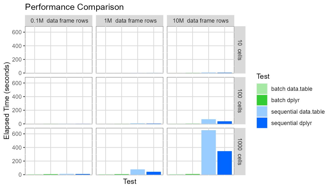
It is clear pivot table creation time is very large when
sequential mode is used for large pivot tables and large
data frames. The pivot table with one thousand cells based on a data
frame containing ten million rows required around 500 seconds to be
created.
Displaying the same chart again, but setting the y-axis maximum to be around 80 seconds:
# clearer captions
library(dplyr)
plotdata <- mutate(scenarios,
                   cellDesc=paste0(cellCount, "  cells"),
                   rowDesc=paste0(
                     recode(rowCount, "1e5"=" 0.1", "1e6"=" 1", "1e7"="10"),
                     "M  data frame rows")
                   )
# plot
library(ggplot2)
colors <- c("#A5E9A5","#33CC33", "#99CCFF","#0066FF")

ggplot(plotdata, aes(x = testName, y = elapsedTimeAvg)) +
  geom_bar(aes(fill=testName), stat="identity", position="dodge") +
  scale_fill_manual(values=colors, name="Test") +
  theme(panel.background = element_rect(colour = "grey40", fill = "white"),
        panel.grid.major = element_line(colour = rgb(0.85, 0.85, 0.85)),
        axis.ticks.x=element_blank(), axis.text.x=element_blank()) +
  scale_y_continuous(expand = c(0.01, 0)) +
  coord_cartesian(ylim = c(0, 84)) +
  labs(x = "Test", y = "Elapsed Time (seconds)", title ="Performance Comparison") +
  facet_grid(cellDesc ~ rowDesc)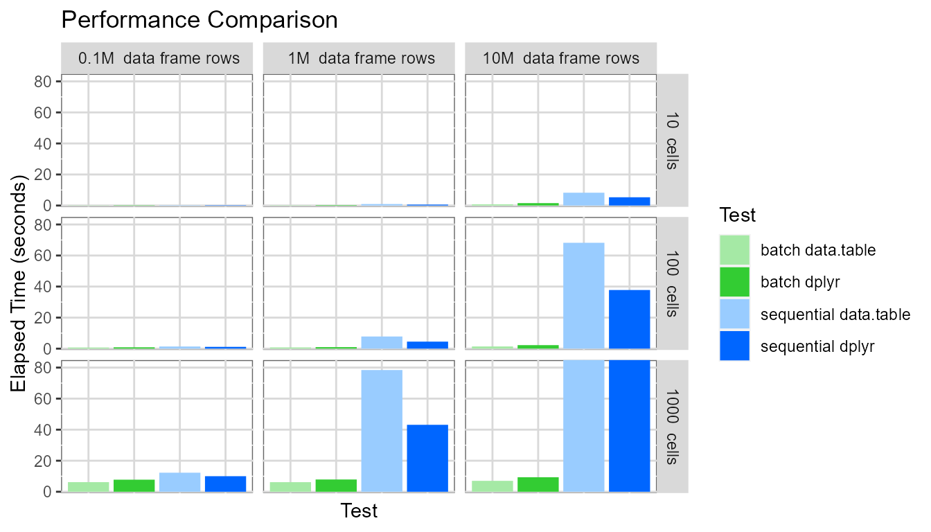
Finally, displaying the same chart again, but setting the y-axis maximum to be around 15 seconds:
# clearer captions
library(dplyr)
plotdata <- mutate(scenarios,
                   cellDesc=paste0(cellCount, "  cells"),
                   rowDesc=paste0(
                     recode(rowCount, "1e5"=" 0.1", "1e6"=" 1", "1e7"="10"),
                     "M  data frame rows")
                   )
# plot
library(ggplot2)
colors <- c("#A5E9A5","#33CC33", "#99CCFF","#0066FF")

ggplot(plotdata, aes(x = testName, y = elapsedTimeAvg)) +
  geom_bar(aes(fill=testName), stat="identity", position="dodge") +
  scale_fill_manual(values=colors, name="Test") +
  theme(panel.background = element_rect(colour = "grey40", fill = "white"),
        panel.grid.major = element_line(colour = rgb(0.85, 0.85, 0.85)),
        axis.ticks.x=element_blank(), axis.text.x=element_blank()) +
  scale_y_continuous(expand = c(0.01, 0)) +
  coord_cartesian(ylim = c(0, 14)) +
  labs(x = "Test", y = "Elapsed Time (seconds)", title ="Performance Comparison") +
  facet_grid(cellDesc ~ rowDesc)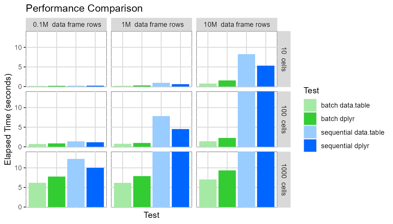
This highlights several interesting points:
- The
batchevaluation mode dramatically outperforms thesequentialevaluation mode. For the pivot table with 1000 cells based on a data frame containing ten million rows, thebatchevaluation mode generates the pivot table approximately 40-90 times faster than thesequentialevaluation mode (7 seconds vs. 650 seconds for data.table and 9 seconds vs. 350 seconds for dplyr). - The pivot table creation time for the
sequentialevaluation mode depends on (pivot table cell count * data frame row count). - The pivot table creation time for the
batchevaluation mode depends only on the pivot table cell count. - For the
sequentialevaluation mode, the dplyr processing library performs slightly better. - For the
batchevaluation mode, the data.table processing library performs slightly better.
The comparatively poor performance of data.table (vs. dplyr) in
sequential evaluation mode is explained as follows: In
sequential mode, two data.table operations are needed for
each cell - the first to identify if any data exists for the cell (using
the data.table .N variable) and the second to calculate the cell
value.
Limits of performance
Very large pivot tables could take a significant amount of time to
calculate, even using batch mode. In the tests above, the
maximum cell generation rate was around 130 cells per second when using
the batch evaluation mode with the data.table processing
library and the none argument check mode. For comparison,
changing the argument check mode to balanced reduces the
maximum cell generation rate to around 100 cells per second.
Now the optimum settings for performance have been identified, a few indicative tests with larger pivot tables can be run:
- 1e7 rows and 1e4 cells requires 66 seconds to generate the pivot table = around 150 cells per second.
- 1e8 rows and 1e4 cells requires 72 seconds to generate the pivot table = around 140 cells per second.
- 1e8 rows and 1e5 cells requires 1050 seconds to generate the pivot table = around 95 cells per second.
- 1e8 rows and 1e5 cells requires 770 seconds to generate the pivot table = around 130 cells per second (for a different data distribution, discussed below).
For very large pivot tables, it is often the case that data won’t exist for every cell (i.e. every combination of row and column headings). The fourth test case above was for a pivot table where around only one-third of the cells contained a value. This pivot table was generated significantly quicker.
From the above four additional tests, it is clear the maximum practical pivot table size (in terms of pivot table creation time) is around 100,000 cells (or possibly a few multiples of that).
The pivottabler package has been designed primarily as a
visualisation tool. Once a pivot table contains 100,000 cells or more it
ceases to become a visualisation tool, i.e. it is not viable for a human
being to look at a table containing 100,000 to 1 million or more cells.
Such use-cases tend to be more like bulk data processing, for which more
optimised data structures such as data frames, tibbles and data.tables
are far better suited.
It is probable some further moderate performance gains could be
achieved by further optimising the pivottabler R code,
however optimisation eventually becomes a game requiring ever more
effort for ever diminishing returns.
Summary
To achieve optimum performance:
- Use the
batchevaluation mode (the default) since it performs orders of magnitudes faster than thesequentialevaluation mode. - Don’t create large pivot tables needlessly.
- Pivot tables having 10,000 cells will take at least one minute to
create, even in
batchevaluation mode. - Pivot tables having more than 100,000 cells will take a relatively
long time to create (more than ten minutes), even in
batchevaluation mode.
- Pivot tables having 10,000 cells will take at least one minute to
create, even in
- Use the data.table processing library with
pivottablerfor data frames with more than ten million rows (but only with thebatchevaluation mode), though take note of the warning above regarding the odd behaviour of data.table in some circumstances. - Reduce the argument check mode for large pivot tables.